Late last year, I had the pleasure of organizing a workshop within the MAIN (Montréal AI & Neuroscience) conference. Its main goal was to expose participants (undergraduate and graduate students alike) to the rich world of computational dynamics and how we can successfully use its tools to reveal insights in our neuroscientific data.

Here’s a link that provides an overview of the workshop can be found here: https://main-educational.github.io/neuroai-dynamical-systems/. You can find my github repo with the workshop materials at this link: https://github.com/dvoina13/mante_and_sussillo_2013. Enjoy!

One of the key components of the workshop was playing around with recurrent neural networks (RNNs) as abstract, simplified models of a neuronal network in the brain. Its units don’t spike, they are instead described by positive real numbers, which is why in our models they are analogous to firing rates. Naïvely, we might implement an RNN using off-the-shelf pytorch:

However, what most neuroscientists use instead is the continuous RNN model which is of course implemented by discretizing (usually via a simple Euler’s method):

So why use this particular formula then?

Discretization blurs the distinction: if you discretize a continuous RNN with Euler, you essentially recover a “normal” RNN — but now you control stability by $\frac{\Delta t}{t}$ and the dynamics are constrained by the underlying continuous system.

The real differences in dynamics between discrete RNNs and continuous RNN
  1. Natural time scale

• Continuous RNNs include an explicit time constant
• Controls how fast hidden states evolve.
• Gives the model an inherent notion of physical time

2. Continuous RNNs connect naturally to neuroscience. They behave like:

• leaky integrators
• firing-rate
• neuronal models

We next went from simple to more complex nonlinear RNNs and analyzed their dynamics behavior, both by simply plotting the dynamics, as well as analytically computing its dynamical behavior through the eigenvectors and eigenvalues of the Jacobian of the system. For example, the Jacobian of the dynamical system $\dot{\textbf{h}} = -\textbf{h} + \textbf{W} \cdot \tanh (\textbf{h})$ is $\textbf{J} = – \textbf{I} + \textbf{W} \cdot \textrm{diag}(1 – \tanh^2(\textbf{h}))$. The eigenspectrum of $\textbf{J}$ determines whether there is stable, unstable or oscillatory dynamics. If there is one or more eigenvalues whose real part $> 0 \Rightarrow$ unstable dynamics; if all eigenvalues have real part <math data-latex=”<0⇒< 0 \Rightarrow stable fixed point; if there are non-zero imaginary parts to the eigenvalues, then there are oscillations. Eigenvectors are important too in better understanding dynamics: they determine the direction in which the trajectory contracts or expands.

Nonlinear RNNs are a game-changer. The nonlinearity allows us to have richer dynamics, not just going to a fixed point or blowing up (e.g., chaotic activity). We look at chaotic activity where the trajectory does not converge to a fixed point or limit cycle (a kind of oscillatory loop in the dynamics), nor does it blow up. Along a chaotic trajectory, the discrete-time Jacobian at each point will usually have some eigenvalues with magnitude greater than 1 (expanding directions) and some less than 1 (contracting directions), with the exact spectrum changing over time. With moderate input signal $\textbf{i}(t)$, the network exhibits rich, complex trajectories, mixing internal chaotic dynamics with input-driven structure. This is the regime exploited in reservoir computing / echo state networks: a simple linear readout of the RNN activity can compute highly non-linear functions of the input.

After this introduction, we dived into a relevant example from the computational neuroscience literature: the Mante and Sussillo paper from 2013¹. Although quite old at this point, this paper has become quite influential in our computational community because it was an early example of inferring neural mechanisms using a network like the RNN.

At that point, 2013, it was also the beginnings of looking more holistically at what the entire population of neurons was doing through some sort of dimensionality reduction technique, as opposed to looking at individual neurons and their tunings. They were not the first to do this, but it was still pretty early days of neuronal population dynamics analysis. In Mante, Sussillo, et. al.’s own words:

“… the observed complexity and functional roles of single neurons are readily understood in the framework of a dynamical process unfolding at the level of the population.” Mante, Sussillo, et. al., 2013

The task they were analyzing was slightly more complex than the classical random-dots discrimination task when animals (monkeys) had to decide whether noisy dots on a screen were moving more to the left or right by making an appropriate saccade (eye movement) in the corresponding direction; rather, animals were given a context signal that indicated whether to look for motion (left versus right), or color (red versus green) prompting them to accumulate information of the relevant stimulus.

Figure 1, Mante, Sussillo, et. al., 2013

Given recordings of hundreds or thousands of neurons, this is a high dimensional signal that can only be visualized through dimensionality reduction, i.e. a changed small-d coordinate space (2- or 3-dimensional) where we can project our neural data and look at the patterns of activity. To achieve this, they used linear regression to define four orthogonal, task-related axes: the axes of choice, motion, color, and context. The projection of the population response onto these axes results in “de-mixed” estimates of these task variables, which are mixed within single neuron activities.

They call this procedure “targeted dimensionality reduction” whereby they go from a high-d space of dimension equal to the number of neurons (each neuron is a dimension in the original state space) to a 4-d space where each dimension corresponds to a task variable. For example, a high value along the choice axis corresponds to a high probability of choosing left (high positive) or right (high negative) direction.

What is interesting is that they can answer a real scientific question with this technique. When they look at the low-d trajectories they see that, regardless of the context, evidence is momentarily accumulated on both the color and motion axis, but the appropriate context-dependent evidence is accumulated towards a choice only along the choice axis. This offers us a crucial insight: the irrelevant, input-dependent activity corresponding to the stimulus that is not contextual is still relevant for the neural activity in the prefrontal cortex — PFC (where they record) and is not filtered early. Other possible models are also ruled out with this visualization (e.g, that the motion and color axes change with respect to the choice axis at each given context).

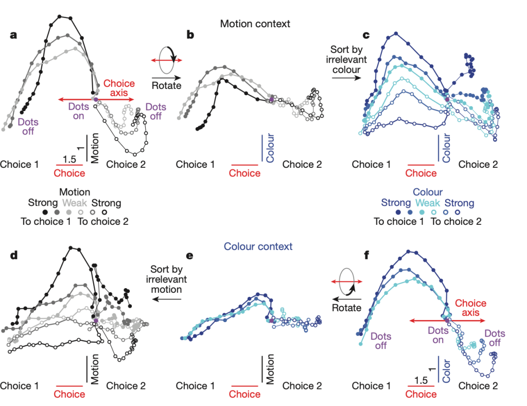
Figure 2, Mante, Sussillo, et. al., 2013:
Dynamics of population responses in PFC.

Finally, these insight can be implemented in an RNN model as described above, where the RNN tries to solve this context-dependent decision-making task just like the animals. This is precisely what I have been trying to implement in my MAIN workshop, showing how the RNN model can capture the same qualitative dynamics of the real neuronal activity as recorded in the monkey brain.

But is there a point to a computational RNN model if we already have gained insights from the dimensionality-reduced data? Well, yes. Because while the real dynamics give us insights and enable us to dismiss particular models, the causative factors for this neuronal activity remain opaque. RNNs give us a unique perspective into their own dynamics because we know the driving differential equations that express the dynamics, so we can better “peer into” their mechanisms much better. While brain dynamics are still pretty opaque (we almost never have access to connectivity data, for example), RNNs are easy to reverse engineer and we have access to all the variables we want.

1. Context-dependent computation by recurrent dynamics in prefrontal cortex, Valerio Mante, David Sussillo, Krishna V. Shenoy & William T. Newsome, Nature volume 503, pages 78–84 (2013)
   ↩︎